Exploring Air Quality in New York: A Predictive Analysis of Ozone Levels Using Environmental Factors

For this analysis, we will explore the airquality dataset, which provides daily air quality measurements in New York from May to September 1973. The dataset includes variables such as Ozone, Solar.R (solar radiation), Wind, Temp (temperature), and the month and day of the observation. Our objective is to analyze the relationships between air quality and weather-related factors, focusing on predicting the levels of Ozone, a key indicator of air pollution.

We will begin by cleaning the data, handling missing values, and performing exploratory data analysis (EDA) to better understand the distribution of variables and their correlations. Subsequently, we will build a linear regression model to predict Ozone levels based on other relevant environmental factors. Through this process, we aim to uncover key insights that could inform further studies on air quality and its environmental determinants.

Loading Data

data("airquality")
str(airquality)

## 'data.frame':	153 obs. of  6 variables:
##  $ Ozone  : int  41 36 12 18 NA 28 23 19 8 NA ...
##  $ Solar.R: int  190 118 149 313 NA NA 299 99 19 194 ...
##  $ Wind   : num  7.4 8 12.6 11.5 14.3 14.9 8.6 13.8 20.1 8.6 ...
##  $ Temp   : int  67 72 74 62 56 66 65 59 61 69 ...
##  $ Month  : int  5 5 5 5 5 5 5 5 5 5 ...
##  $ Day    : int  1 2 3 4 5 6 7 8 9 10 ...

head(airquality)

##   Ozone Solar.R Wind Temp Month Day
## 1    41     190  7.4   67     5   1
## 2    36     118  8.0   72     5   2
## 3    12     149 12.6   74     5   3
## 4    18     313 11.5   62     5   4
## 5    NA      NA 14.3   56     5   5
## 6    28      NA 14.9   66     5   6

Data Cleaning and Handling Missing Values

First, we begin by inspecting the airquality dataset and handling the missing values. The Ozone variable contains some missing values, which we will address before proceeding with further analysis.

Check for missing values in Ozone

sum(is.na(airquality$Ozone))  # Count of missing values

## [1] 37

Remove rows with missing values

cleaned_data <- na.omit(airquality)
head(cleaned_data,5)

##   Ozone Solar.R Wind Temp Month Day
## 1    41     190  7.4   67     5   1
## 2    36     118  8.0   72     5   2
## 3    12     149 12.6   74     5   3
## 4    18     313 11.5   62     5   4
## 7    23     299  8.6   65     5   7

Alternatively, impute missing values with the mean (if preferred)

• airquality$Ozone[is.na(airquality$Ozone)] <- mean(airquality$Ozone, na.rm = TRUE)

The dataset contains missing values, particularly in the Ozone variable. We address these missing values by removing rows with NA values using na.omit() or by imputing missing values with the mean of the Ozone variable. This ensures we have a complete dataset to work with.

Exploratory Data Analysis (EDA)

Next, we perform exploratory data analysis to understand the distribution of variables and relationships between them.

library(ggplot2)
ggplot(cleaned_data,aes(Ozone)) +
  geom_histogram(bins = 30,colour = "red") +
  ggtitle("Histogram of Ozone Levels")

ggplot(cleaned_data,aes(Temp))+
  geom_histogram(bins = 30,colour = "blue") + 
  ggtitle("Histogram of Temperature Levels")

ggplot(cleaned_data,aes(Temp,Ozone)) +
  geom_point() +
  ggtitle("Ozone vs Temperature")

ggplot(cleaned_data,aes(Solar.R,Ozone)) +
  geom_point() +
  ggtitle("Solar Radiation vs Ozone ")

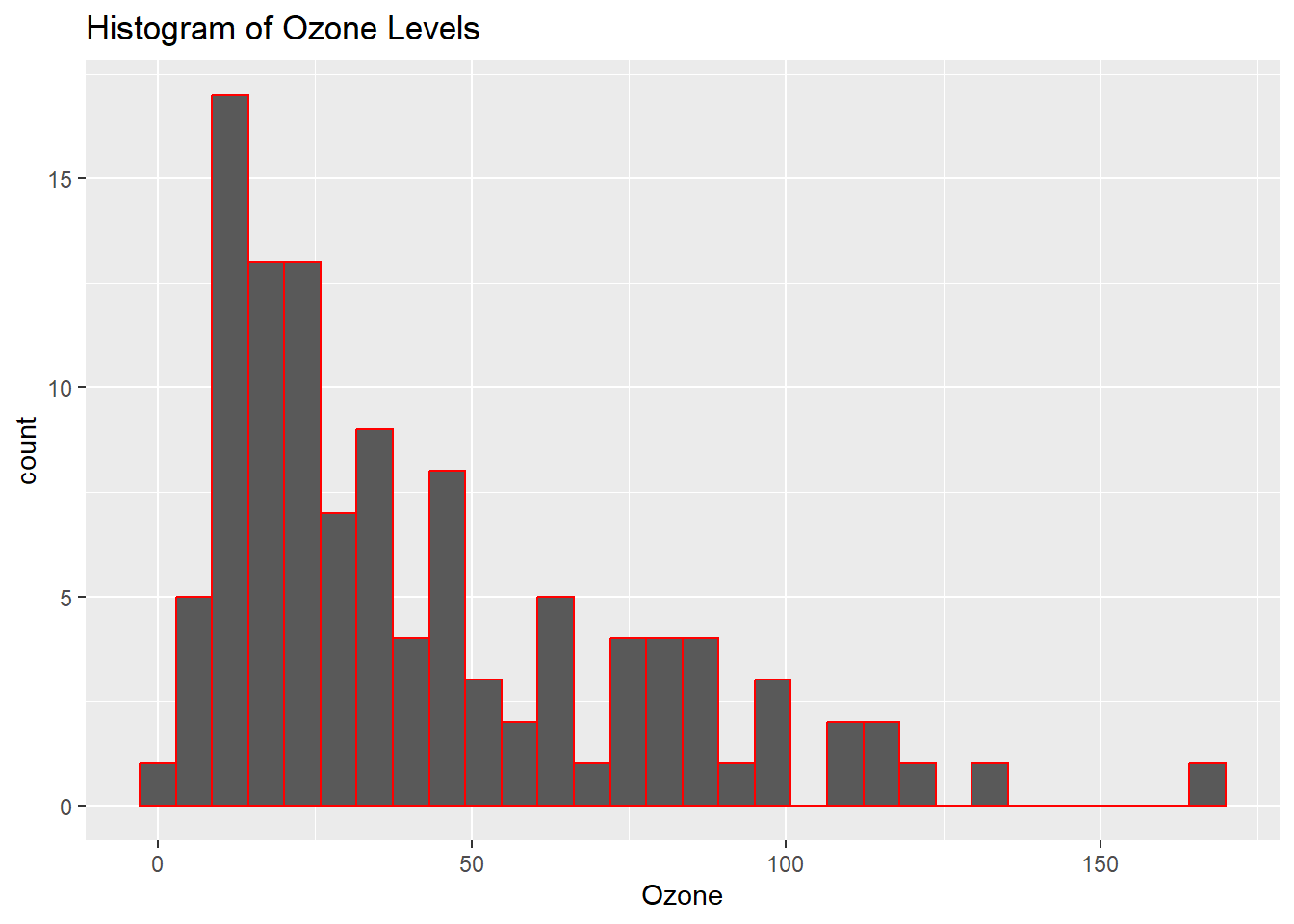
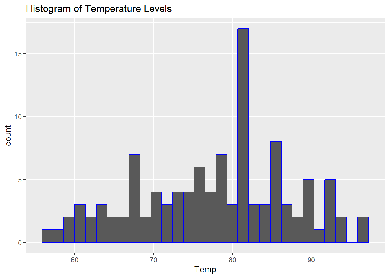
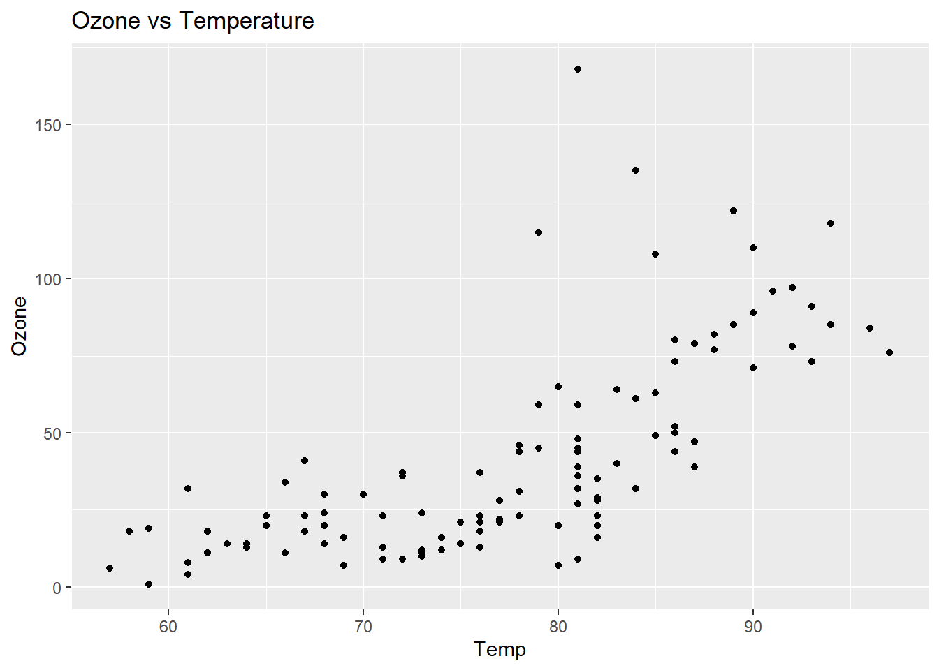
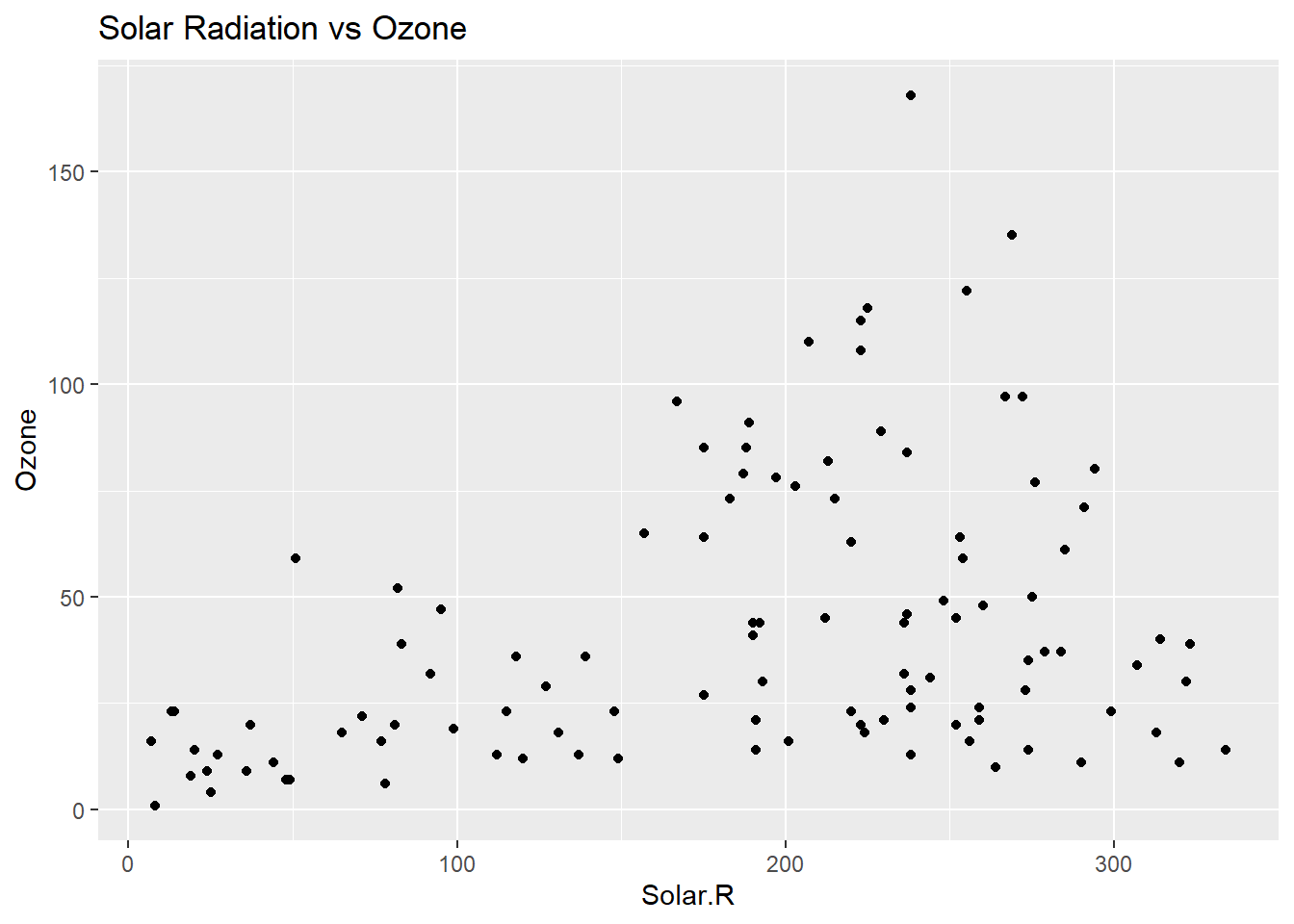In the EDA phase, we generate summary statistics and visualizations to understand the data better. Histograms of Ozone and Temp show the distribution of these variables, while scatter plots reveal the relationships between Ozone and other variables like Temp and Solar.R. We also calculate the correlation matrix to identify any linear relationships between numeric variables. These steps help us understand the patterns in the data before building predictive models.

Building a Linear Regression Model

After cleaning and exploring the data, we build a linear regression model to predict Ozone levels based on environmental factors like Solar.R, Wind, and Temp.

model <- lm(Ozone ~ Solar.R + Wind + Temp, data = cleaned_data)
summary(model)

## 
## Call:
## lm(formula = Ozone ~ Solar.R + Wind + Temp, data = cleaned_data)
## 
## Residuals:
##     Min      1Q  Median      3Q     Max 
## -40.485 -14.219  -3.551  10.097  95.619 
## 
## Coefficients:
##              Estimate Std. Error t value Pr(>|t|)    
## (Intercept) -64.34208   23.05472  -2.791  0.00623 ** 
## Solar.R       0.05982    0.02319   2.580  0.01124 *  
## Wind         -3.33359    0.65441  -5.094 1.52e-06 ***
## Temp          1.65209    0.25353   6.516 2.42e-09 ***
## ---
## Signif. codes:  0 '***' 0.001 '**' 0.01 '*' 0.05 '.' 0.1 ' ' 1
## 
## Residual standard error: 21.18 on 107 degrees of freedom
## Multiple R-squared:  0.6059,	Adjusted R-squared:  0.5948 
## F-statistic: 54.83 on 3 and 107 DF,  p-value: < 2.2e-16

Model Summary

The linear regression model was fitted with Ozone as the dependent variable and Solar.R, Wind, and Temp as independent variables.

##Key Findings:

• Intercept: The intercept is -64.34, which represents the estimated ozone level when all predictors (solar radiation, wind, and temperature) are zero.

• Solar.R: The coefficient for Solar.R is 0.05982, indicating that for each unit increase in solar radiation, the ozone level is expected to increase by approximately 0.05982 units. The p-value of 0.01124 suggests that solar radiation is a statistically significant predictor of ozone levels at the 5% significance level.

• Wind: The coefficient for Wind is -3.33359, implying that for each unit increase in wind speed, the ozone level is expected to decrease by about 3.33 units. The p-value of 1.52e-06 is highly significant, indicating that wind is a strong predictor of ozone levels.

• Temp: The coefficient for Temp is 1.65209, meaning that for each unit increase in temperature, the ozone level is expected to increase by approximately 1.65 units. The p-value of 2.42e-09 indicates that temperature is also a highly significant predictor.

##Model Fit:

• Residual Standard Error: The residual standard error of 21.18 tells us about the typical size of the residuals (i.e., the typical difference between the observed and predicted ozone levels). A lower value would suggest a better fit, but this value is relatively moderate.

• R-squared: The Multiple R-squared value of 0.6059 indicates that approximately 60.6% of the variability in ozone levels is explained by the model. The Adjusted R-squared of 0.5948 adjusts for the number of predictors and is slightly lower, but still suggests a reasonably good fit for the data.

• F-statistic: The F-statistic is 54.83 with a p-value of < 2.2e-16, which indicates that the model as a whole is statistically significant, meaning the independent variables together do a good job of explaining ozone levels.

Interpretation:

The results suggest that:

• Temperature, solar radiation, and wind all have significant impacts on ozone levels in New York.
• Solar radiation and temperature are positively related to ozone levels, meaning that higher solar radiation and warmer temperatures lead to higher ozone concentrations.
• Wind speed, on the other hand, has a negative relationship with ozone levels, suggesting that stronger winds are associated with lower ozone concentrations.
• The model has a decent fit (with an R-squared of around 60%), but there may still be unexplained variability, which is typical in environmental datasets. Further refinement or additional variables could potentially improve the model’s predictive power.

Model Diagnostics and Evaluation

To ensure the model is valid, we perform diagnostic checks, including evaluating the residuals to confirm the assumptions of linear regression.

par(mfrow = c(2, 2))
plot(model)

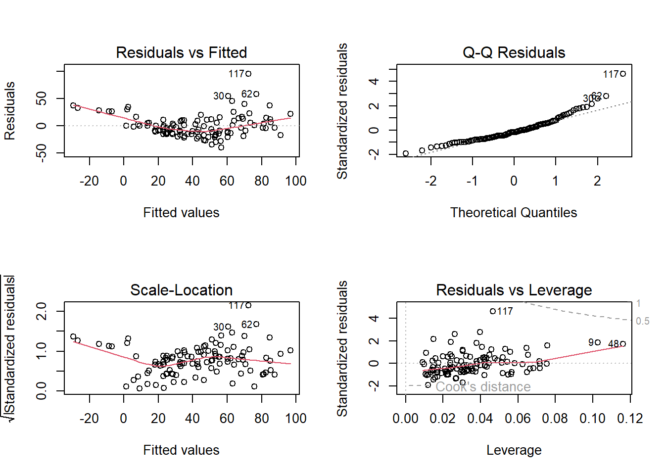
• Q-Q Residual plot - Residuals are approximately normal, and the normality assumption holds.